This is the project website & blog of MIRLCAuto: A Virtual Agent for Music Information Retrieval in Live Coding, a project funded by the EPSRC HDI Network Plus Grant - Art, Music, and Culture theme.
Towards Learning My Musical Taste When Retrieving Sounds From Freesound
28 Dec 2020 • Anna Xambó • Post a comment
In this blog post, I will explain the direction undertaken towards solving the first machine learning task of the project: learning a personal musical taste when retrieving sounds from Freesound. This task is based on the question of whether a person likes or not the retrieved sounds from the online database distinguishing them between 'good' and 'bad' sounds.
In particular, I will focus on explaining the process of (1) creating a manually annotated dataset for training and testing; (2) identifying suitable audio descriptors; and (3) training a suitable model using a multilayer perceptron (MLP) neural network classifier that recognises my musical taste.
The code is available in SuperCollider here and is based on the following SuperCollider extensions:
- Freesound.quark
- MILRC 2.0
- Flucoma
Creation of a manual dataset #
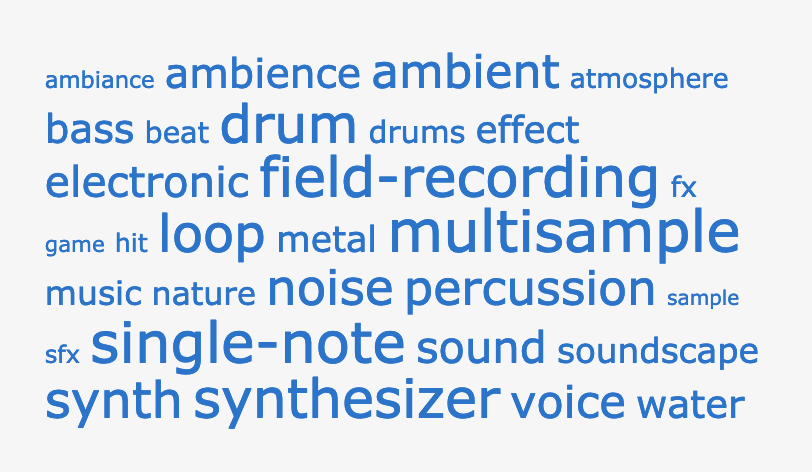
The Freesound database has 481,305 sounds at the time of writing this blog post. For this task, the idea was to create a small dataset, which should be representative of the database. There was a selection of 100 sounds for the training dataset and 30 sounds for the testing dataset. A range of sounds was selected from the most popular tags (see Fig. 1), including melodic sounds, rhythmic sounds, melodic-rhythmic sounds, ambience sounds, and sound effects, among others. In particular, the following tags were used:
- Electronic (10 sounds training, 3 sounds testing)
- Bass (10 sounds training, 3 sounds testing)
- Voice (10 sounds training, 3 sounds testing)
- Drum (10 sounds training, 3 sounds testing)
- Loop (10 sounds training, 3 sounds testing)
- Noise (10 sounds training, 3 sounds testing)
- Soundscape (10 sounds training, 3 sounds testing)
- Ambience (10 sounds training, 3 sounds testing)
- Metal (10 sounds training, 3 sounds testing)
- Effect (10 sounds training, 3 sounds testing)
For each tag, the first 10 results were selected. However, repeated sounds or very similar sounds (e.g. from the same collection), which were in the same category, or repeated across multiple categories, were skipped to obtain 130 unique sounds. In the rare situation of finding sounds with no descriptors (e.g. long sounds), the sounds were also ignored.
Once 130 sounds were selected, they were annotated with the label "good" or "bad", depending on the personal musical taste. You can find an example of both annotated training-input.txt and testing-input.txt datasets with the sounds listed by their Freesound identification number (aka "id") in the following link:
The next step was to identify suitable audio descriptors and automatically complete the datasets with their corresponding audio descriptor values.
Identifying suitable audio descriptors #
Approach 1 #
For the first approach, a few audio descriptors were used, related to the pitch, rhythm, brightness and noisiness of the sound samples. This decision was informed by the literature (Navarro and Ogborn, 2017; Stewart et al. 2019; Stewart et al. 2020) and fundamental music characteristics. Several audio descriptors are available in Freesound (https://freesound.org/docs/api/analysis_docs.html) via the Essentia algorithms (https://essentia.upf.edu). The following audio descriptors were used, including both mean and variance:
- lowlevel.pitch.mean and lowlevel.pitch.var, which measure the pitch value of a sound.
- rhythm.bpm, which measures the bpm value of a sound.
- lowlevel.spectral_centroid.mean and lowlevel.spectral_centroid.var, which measure the brightness of a sound.
- lowlevel.spectral_flatness_db.mean and lowlevel.spectral_flatness_db.var, which measure the noisiness of a sound.
- lowlevel.pitch_instantaneous_confidence.mean and lowlevel.pitch_instantaneous_confidence.var, which measure the strength of the pitch value, where a low value indicates that the sound has a 'weak' pitch, whilst a high value indicates that the sound has a 'strong' pitch.
In an iterative process, the above 9 audio descriptors were tested for training a multilayer perceptron neural network (explained in the section "Training a suitable model"). However, the accuracy results were modest (50%-57% accuracy). After plotting the histograms and boxplots of all the above descriptors (see Fig. 2), it was clear that the most visible differences were among the audio descriptors of:
- Spectral flatness (mean and variance)
- Pitch confidence (mean and variance)
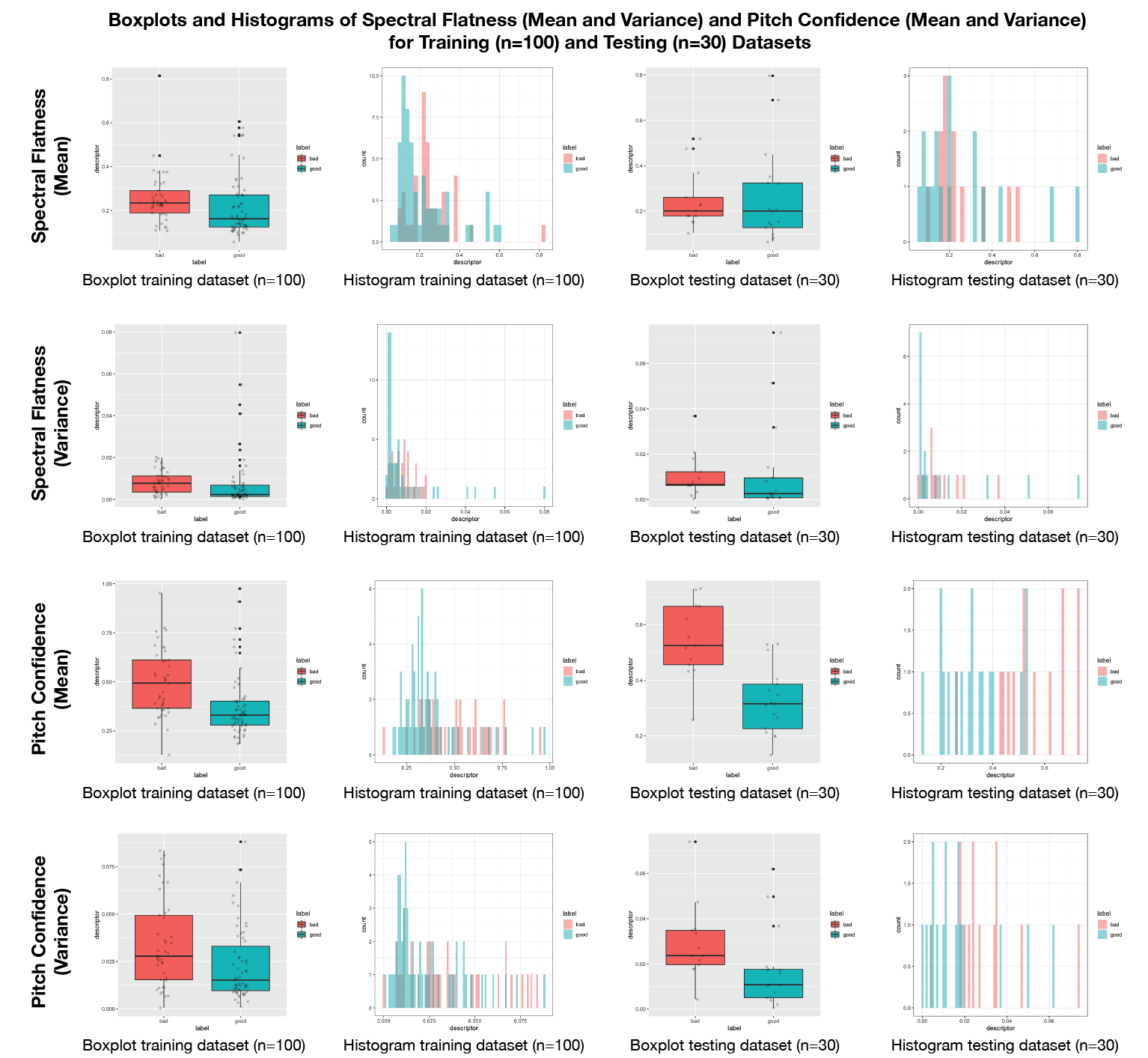
When only selecting these 4 audio descriptors (mean and variance of flatness and pitch confidence), an accuracy of 73% was achieved. A multilayer perceptron neural network was used of 1 hidden layer of 3 nodes and the Relu activation function. Although the result was more positive than the previous attempt, a second approach was undertaken, explained in the next section.
Approach 2 #
For the second approach, the Mel-frequency cepstral coefficients (MFCCs) audio descriptors was used. MFCCs are widely used in automatic speech and speaker recognition for describing timbrical properties of audio signals.
When using 26 audio descriptors (mean and variance of the 13 MFCCs), the accuracy results obtained were of 76%-83%. A multilayer perceptron neural network was used (explained in the section "Training a suitable model").
You can find an example of both annotated training-input-complete.txt and testing-input-complete.txt datasets with the sounds listed by their Freesound identification number (aka "id") in the following link:
Automatic completion of the dataset #
For both rounds and both training and testing datasets, the following code was used to autocomplete the audio descriptor values for each of the selected sounds from the original manual dataset:
Training a suitable model #
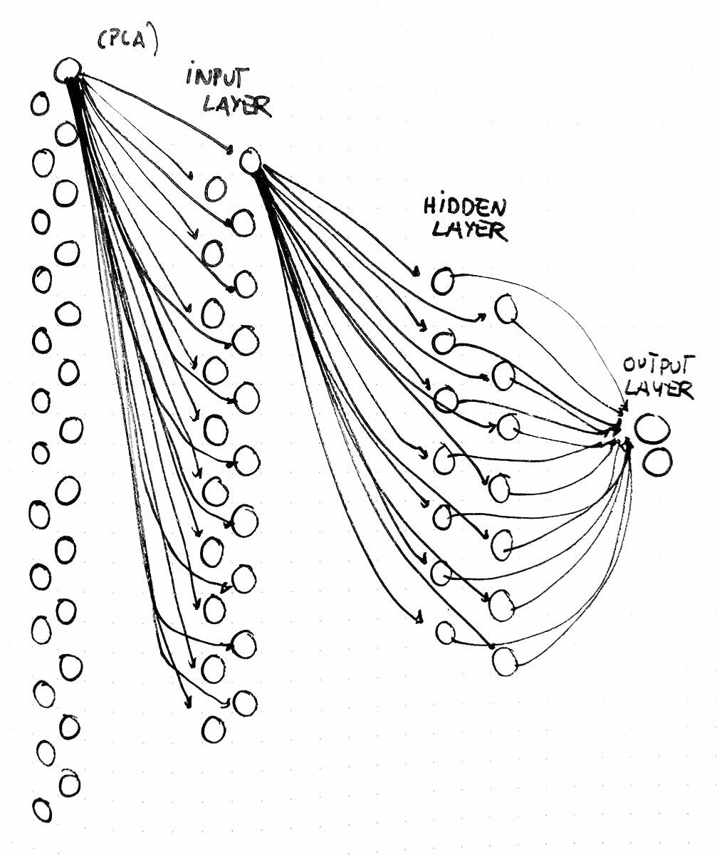
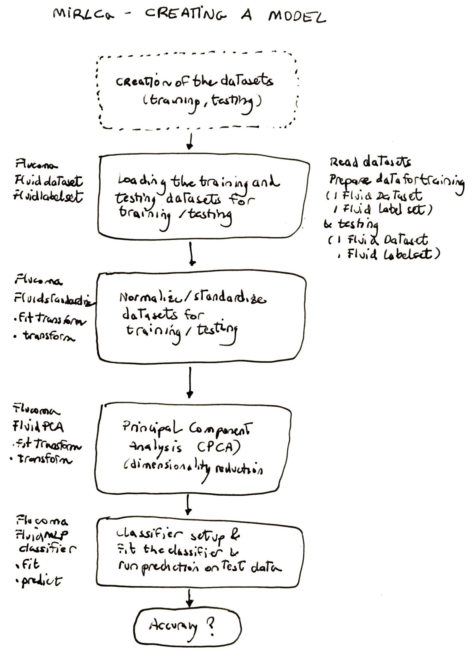
An iterative process was followed to find a suitable set of audio descriptors as well as a suitable multilayer perceptron neural network to train the classifier. In sum, the best result was obtained using 26 MFCCs (mean and variance). The 26 audio descriptors were reduced to 20 dimensions via the Principal Component Analysis (PCA) method. The MLP was configured with 1 hidden layer of 14 nodes, a learning rate of 0.01 and the Relu activation function. Figure 3 illustrates the configuration of the MLP neural network. Figure 4 shows a block diagram of the steps required to prepare the data for the classifier.
You can find the code implemented in the MIRLCa SuperCollider extension as well as a step-by-step tutorial in the SuperCollider file manual-training-musical-taste-classifier.
The video demos MIRLCa Performance Mode and MIRLCa Training Mode are based on this classification model.
Acknowledgements #
I am very grateful to Gerard Roma for his mentoring role in the project.
References #
- Navarro, Luis and Ogborn, David. “Cacharpo: Co-performing Cumbia Sonidera with Deep Abstractions.” Proceedings of the 2017 International Conference on Live Coding (Morelia, Mexico, 4–8 December 2017).
- Stewart, Jeremy and Lawson, Shawn. “Cibo: An Autonomous TidalCyles Performer.” Proceedings of the Fourth International Conference on Live Coding (Madrid, Spain: Medialab Prado / Madrid Destino, 16–18 January 2019).
- Stewart, Jeremy, Lawson, Shawn, Hodnick, Mike and Gold, Ben. “Cibo v2: Realtime Livecoding A.I. Agent.” Proceedings of the 2020 International Conference on Live Coding (Limerick, Ireland: University of Limerick, 5–7 February 2020), pp. 20–31.